Overview of Data Assimilation
The earth, the weather, the atmosphere and the oceans of the world are prime examples of highly nonlinear dynamical systems. Understanding them using physics behind their evolution in time relies on governing physical laws of conservation(mass, momentum,..), using numerical simulations. But these are infinite dimesnional systems, highly nonlinear, chaotic and predicting them means controlling the error in our estimate of their present, and future behaviour. To make the numerical representation of such systems follow the true system, we need a method to consolidate the real observations into the numerical models, so that what the numerical models shows/predicts is a good approximation of reality. Data assimilation algorithms are necessary to track or estimate the hidden state of chaotic systems through partial and noisy observations. Variational data assimilation aims to find a the best trajectory of the dynamical system which minimizes a certain cost function.
Problem statement: Can neural network models replace data assimilation for a cheaper/faster alternative?
For an observation window $i$ where the sequence of observations $Y^i=\left(y^i_0,y^i_1,…y^i_n\right)$ on $\left(\Omega^i_n\right) \in \Omega$ is given, we want to find the optimal trajectory $X^i=\left(x^i_0,x^i_1,…x^i_n\right)$ of the true system that minimizes the following cost function.
$$\mathcal{U}(x^i_0,x^i_1,…x^i_n)=\sum_{k=1} \alpha_{dyn} | x_k - \mathcal{M}(x_{k-1}) |^2+ \alpha_{ob} |y_i-\mathcal{H}(x_i)|^2$$
This is the weak-4dvar cost function which needs ot be minimized. The dynamical systems $ \mathcal{M} $, the dynamical propagator which takes the system state $x_k$ to $x_{k+1}$. The above weak formulation of the 4dvar problem accounts for additional model errors in the dynamical system as the dynamics is not perfect, hence there dynamical cost term.
The first term minimizes the depatures from a pure model trajectory since the aim to find a trajectory close to the model trajectory while accounting for the model error- a part we refer to as ‘the dynamical cost’. The second term makes the trajectory fit to the obsrvations and is referred as ‘observation cost’.
Introducing Neural Data Assimilation using 4DVarNet
What if we have a dataset of the optimal states and their corresponding observations, can we train a neural network to learn the mapping from the observations to the optimal state? In the supervised setting, we something similar happens when we have access to a large dataset. But simple inversion from observation to full state is an ill-defined problem, so the model learn a representation of the data which acts as a regularization term.
4DVarNet is trained to learn the mapping from the observations to the optimal state, while also learning representation term via a term called GIBBS neural network. This is an autoencoder based network whose input and outputs are the same.
An schematic of the 4DvarNet Architecture
At the core of the 4VarNet architecture is a parameterized 4dvar cost function that we want to learn.
$$\mathcal{U_{\Phi}}= \alpha_{dyn} | X^{i} - \Phi({X^i}) |^2+ \alpha_{ob} |Y^i-\mathcal{H}(X^i)|^2$$
Where we compactify the notations for the time series and $i$ here is the index of assimilation window. Note, that this cost has two parts, the first part learns a representation of the data, while the second part ensures that the observations are matched to the state. There is no background term in this formulation, as the network is expected to learn the correlations from the data.

The solver of this cost function is another neural network that learns the mapping from the observations to the optimal state. This is parameterized by an LSTM whose input is a gradients. We can see this solver as doing meta-learning. The solver is trained to minimize the cost function using a gradient-based descent algorithm, which is similar to the optimization process used in 4dvar.
The parameterized cost function and it’s solver are trained together in an end-to-end manner, allowing the network to learn the optimal mapping from the observations to the optimal state. The loss function that trains the whole architecture is the mean squared error between the predicted state and the true state, given by,
$$\mathcal{L}(X^i, \hat{X}^i) = \frac{1}{N} \sum_{i=1}^{N} | X^i - \Psi_{\Phi,\Gamma}(Y^i,{X}^0) |^2$$
where,
$ \Phi, \Gamma,$ are the parameters of the GIBBS neural network and the solver neural network respectively, $Y^i$ is the observations over an assimilation window indexed by $i$, ${X}^0$ is the initial guess of the state, and $\Psi_{\Gamma,\Phi}$ is the mapping learned by the 4DVarNet architecture.
Interestingly, we just need observations and the true states, not the optimization solutions since the goal of the optimization itself is to revove the true field within the limits of the model/observation errors.
Training and inference:
We have $(Y^i, X^i)$ define as above for the input and target pair for training. The input to the network is generally $Y^i$ in the standard architecture of 4DVarNet. In my case, the network starts with an initial guess of the state $X^i_0$ which is then used to compute the model trajectory $X^i$.
Usually, the IC can be a zero field or a random field, but in my case, I generate a slightly perturbed version of the true state $X^i_0$ as the initial guess. This is done by displacing the true state field in a coherent manner such that the features are preserved and are physical.
During inference, we can use the trained network to predict the optimal state given the observations and some initial conditions. Inprinciple, we can generate multiple predictions by sampling from the initial condition distribution, which can be a Gaussian distribution with mean as the initial guess and some variance. This gives us an ensemble of predictions which can be used for uncertainty quantification.
Quasi-geostrophic model: our choice of the underlying system
To rigorously evaluate and benchmark state estimation algorithms, it is crucial to move beyond over-simplified dynamical systems like the Lorenz-63 or Lorenz-96 models, which are low-dimensional ODEs (3 and 40 dimensions, respectively). At the same time, we need models that are computationally tractable and can be used to test the performance of data assimilation algorithms.
With recent trends of deep learning, traditional data assimilation problems that need adjoint computation may bypass this step by leveraging AD(automatic differentiation)- the work-horse of modern machine learning. The Quasi-Geostrophic (QG) model offers a more realistic and challenging alternative. As a PDE-based model, the QG system captures essential features of large-scale geophysical fluid dynamics while remaining computationally tractable. It serves as a model of intermediate complexity, bridging the gap between toy models and full-scale numerical weather prediction systems.
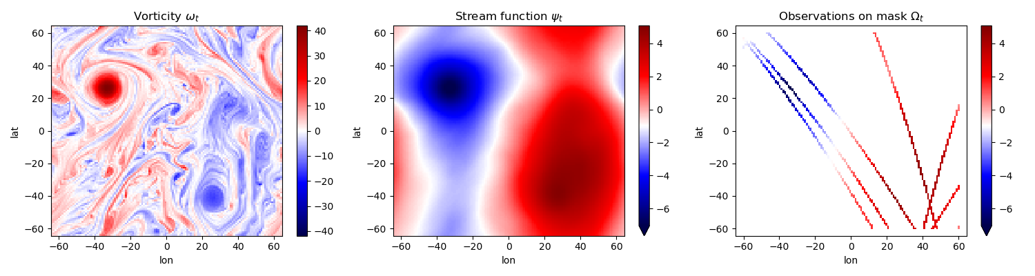
In the QG model, the vorticity field is the fundamental dynamical variable, evolving under nonlinear advection and forcing, and governed by conservation laws. Observations, however, are typically taken in the streamfunction space, which is related to vorticity through an elliptic inversion (a form of diagnostic relationship). This setup introduces a realistic observation operator and offers a natural framework for exploring the performance of data assimilation techniques in the presence of model and observation noise. The QG model is thus particularly well-suited for testing advanced machine learning and deep learning methods for data assimilation I started out with the codes of Hugo Frezat for QG, but I have made significant changes to the code to make it compatible with the weak-4dvar problem and to integrate it with neural ode package.
The Domain is 2D periodic, $\left[0,2 \pi\right)^2$, $\omega $: Vorticity field, $\psi$: Stream-function field.
$$\frac{\partial \omega}{\partial t}+ J(\psi, \omega)= \nu \nabla^2 \omega - \mu \omega - \beta \partial_x \psi ,, \quad \omega = \nabla^2 \psi , \quad $$
The PDE has PBC and we use psueod-spectral methods to solve them( all in pytorch.) These observations are available on masks which have been obtained from Nadir Satelite altimetry tracks. The nature of these observations are realistic- they are really quite sparse!
We finally create a dataset of observations and the true states, which can be used to train the 4DVarNet architecture. The dataset is created by simulating the QG model and generating observations at different times. The observations are then used to train the 4DVarNet architecture to learn the mapping from the observations to the true states.
Results (Work in progress)
The standard 4DVarNet architecture only uses the observations as the input, and intializes the states from it. We refer to this as 4Dvarnet-No-IC. The 4DVarNet architecture where we provide additional guess for the initial conditions is referred to as 4DVarNet-IC. Using a simple metric called $\mu=1-\frac{RMSE(X)}{RMS(X)}$. The RMSE is the root mean square error between the predicted state and the true state, and RMS is the std. of the true state. When $\mu=1$, the model is perfect, and when $\mu=0$, the errors are of the same order of the natural variability of the field X.
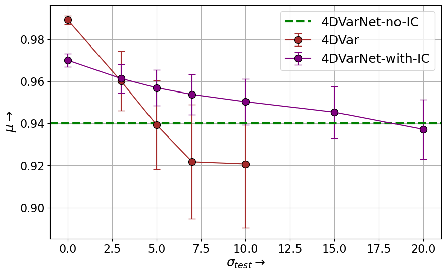
The results of the 4DVarNet architecture are compared with the standard weak-4DVar algorithm, ( both solve the weak-4dvar problem). The results show that the 4DVarNet-IC architecture performs better than the 4DVarNet-No-IC architecture, which is expected since the initial guess is closer to the true state. The results also show that the 4DVarNet architecture is able to learn the mapping from the observations to the true states, and can be used for data assimilation and uncertainty quantification.