General overview of the problem
Weather, ocean, atmosphere to name a few are physical systems in numerical weather prediction which have huge degrees of freedom and are modelled uisng coupled nonlinear PDEs. When a general nonlinear dynamical system is chaotic, two nearby states evolve and deaprt from each other and predictability skill of such systems is very much limited to time-scales which are fixed by the exponents called lyapunov exponents. In practice, purely model based prediction is impossible for such systems as unavoidable errors in initial conditons, model parameters and error in the model equations themselves get quickly amplifiled, making the error huge and essenstially of the size of the attractor (Palmer(2013)).
Data assimilation for dynamical systems
For a dynamical system evolving in real time where the full state is not observed or is observed partially and indirectly, bayesian formalism combines the model outputs with the serially arriving observations allowing one to reasonably estimate the state at time t along with their related uncertainty. Since estimating the full density is impossible in high-dimensions, important statistics describing the pdf are estimated such as mean and covariance and how they evolve in time. Various data assimilation algorithms differ in their specific assumptions and approximations in order to optimally combine the model and the observations making the sequential estimation of such statistics computationally tractable in high-dimensions. Two popular class of such sequential filters are ensemble kalman filters and particle filters.
Bayesian filtering algorithms for data assimilation
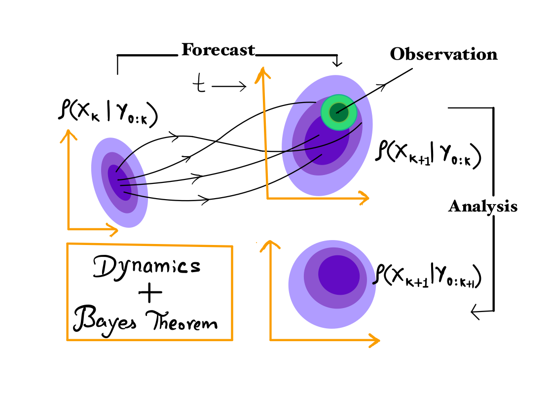
Bayesian filtering is defined as the sequential estimation of the conditional distribution in phase space of the state of a physical system coming from an assumed model taking into account the likelihood of new information arriving from the observations (Cohen(1997)). Filtering is followed by prediction, where the goal is to predict the the evolution of the system and it’s flow dependent uncertainty accounting for possible source of errors which result may grow at later time in future. Below is a schematic picture of a bayeisan filtering mechanism.

At a given time $k$ , the probability density distribution of the true state conditioned on observations upto time $k$ is called the analysis probability density. This is then propagated in time by solving fokker-planck equation, or by using monte-carlo methods to integate the ensembles representing the distribution to obtain prior distribution at time $k+1$, called forecast probability density distribution at time $k+1$, before using the information about the observation $y_{k+1}$. Assuming that given $x_{k+1}$, the observations $y_{K+1}$ is conditionally independent of all previous observations and states, we get the likelihood for the observation $y_{k+1}$ is obtained using the observation model and the measurement noise distribtution is given by $\rho(y_{k+1}|x_{k+1})$. Using bayes' theorem, we have
$$\rho\left(x_{k+1}|Y_{k+1}\right)=\frac{\rho\left(y_{k+1}|x_{k+1}\right)\rho\left(x_{k+1}|Y_{k}\right)}{ \rho\left(y_{k+1}|Y_{k}\right)}$$
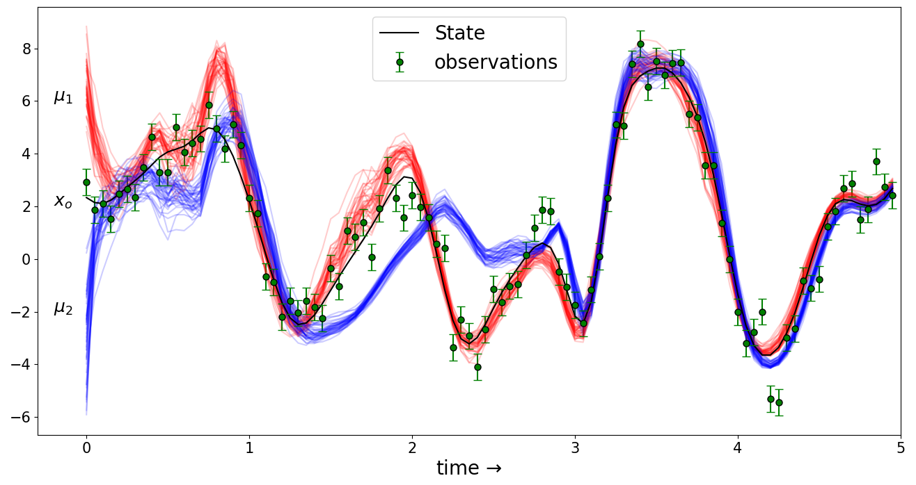
since the true state is unknown, all filtering algorithms makes an arbitraty choice for $\rho(x_0)$ at the time of filter initialization. It becomes crucial that these distributions become independent of the initial choice used in initializing the filter so that quantities estimates using the posterior are eventually independent of our arbitrary and often wrong choice of $\rho(x_0)$. As an example, the following picture demonstrates how stability looks like in one of the component out of the whole state vector,

where we have two different initial distribution $\mu_1$ and $\mu_2$ both of which are far from $x_0$, the true initial condition. Over many assimilation, the two posterior ensembles starting with different initial distribution are seen to come closer to each other.
Definition of filter stability
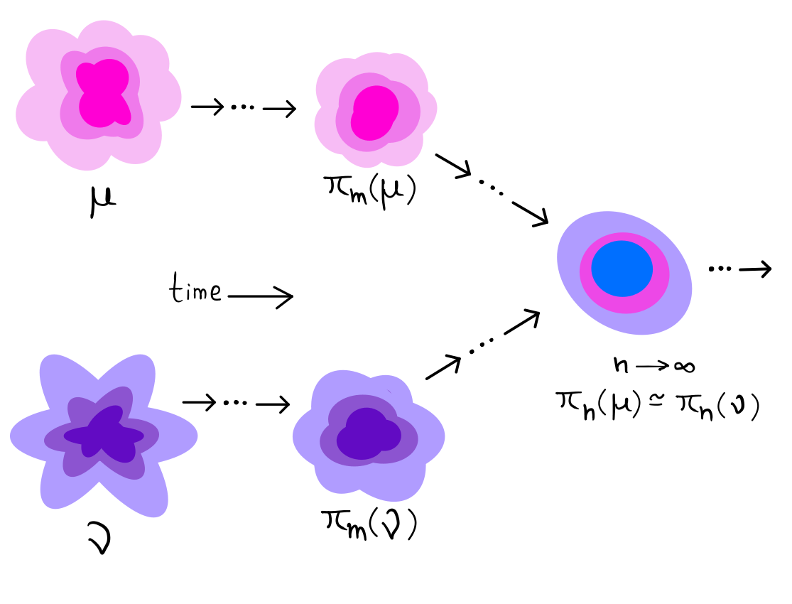
Filter stability is the property that the posterior distribution computed sequentially over long time is independent of the choice of the distribution at $k=0$ used to initialize the filtering algorithm. The rate at which the filter achieves this independece, the better are the estimates of various quantities which utilize the posterior distribution.
Mathematically, we can define it using a distance $D$ on the space of probaility distributions $P(\mathcal{R}^d)$. Given two different initial distributions {$\nu_1, \nu_2$} for $x_0$ with $\hat\pi_n(\nu_1)$ and $\hat\pi_n(\nu_2)$ being the posterior obtained after assimilating all observation $y_{1:n}$ upto time $n$, then for filter stability to hold, we have $$\lim_{n\to\infty}\mathbf E[D(\hat\pi_n(\nu_1), \hat\pi_n(\nu_2))] = 0$$
where, $D$ is a distance on $P(\mathcal{R}^d)$, the space of probability measures on $\mathcal{R}^d$ and the expectation is over observation noise accounting for different noise realizations (mandal(2021)).
 In our work, we have chosen Sinkhorn distance, a distance well motivated by the ideas of optimal transport, which has several merits over other distances such as total variation, apart from being computationally cheaper. This distace utilizes two samples from their respective distributions in order to compute the distance between them upto it’s statistical errors.
We have used Sinkhorn distance to compute these distance. I talk about this distance in another post.
References
[1] Carrassi, A., Bocquet, M., Bertino, L., Evensen,Data assimilation in the geosciences: An overview of methods, issues, and perspectives
[2] G. Evensen,The Ensemble Kalman Filter: theoretical formulation and practical implementation,Ocean Dynamics.
[3] Kevin K W Cheung,A review of ensemble forecasting techniques with a focus on tropical cyclone forecasting,Meteorological Applications, Royal Meteorological Society.
[4] Mandal, Pinak and Roy, Shashank Kumar and Apte, Amit,Stability of nonlinear filters-numerical explorations of particle and ensemble Kalman filters, 2021 Seventh Indian Control Conference (ICC).
[4] Aude Genevay, Thesis-Entropy-regularized optimal transport for machine learning,Paris Sciences et Letters, 2019.