Instability property of a dynamical system and data assimilation
Instability properties of a chaotic nonlinear dynamical system are characterized globally by lyapunov exponent and locally by lyapunov vectors, which correspond to the directions associated with those rates. Unstable subspaces of a system has been shown to improve forecasts in ocean-atmosphere coupled models when the assimilation takes into account \cite{Vannitsem(2016)}. When a time evolving system is only accessible via noisy and sparse observations and with no information of the initial conditions, identifying a trajectory is extremely difficult using only the model and methods of nonlinear filtering provide best estimates of the true state and help us estimate the underlying trajectory the system evolves on with some uncertainty estimate. The best estimates over time does not constitute a dynamical trajectory and but is always near the true trajectory in some distance metric. We formulated this problem into using the filter estimate over time as a proxy of the true trajectory perturbed by the error statistics.
Covariant Lyapunov Vectors
Covariant lyapunov vectors are non-orthogonal basis to the tangent space of a dynamical system, where the $i^{th}$ clv orresponds to the direction along which an infinitesimal error grows or decays with the rate which is equal to the lyapunov $\lambda_i$ in the forward and the time reverse ddynamics respectively. They are covarinat, time-invariant and their computation is costlier than the commonly used backward lyapunov vectors which are orthogonal by construction. CLVs encode more information in terms of theri mutual angle, which is not present in other orthogonal vectors. Accessing this required their computation which is slightly more involved the backward lyapunov vectors, whic are usually the product of Benettin’s algorithm extensively used to compute lyapunov exponents.
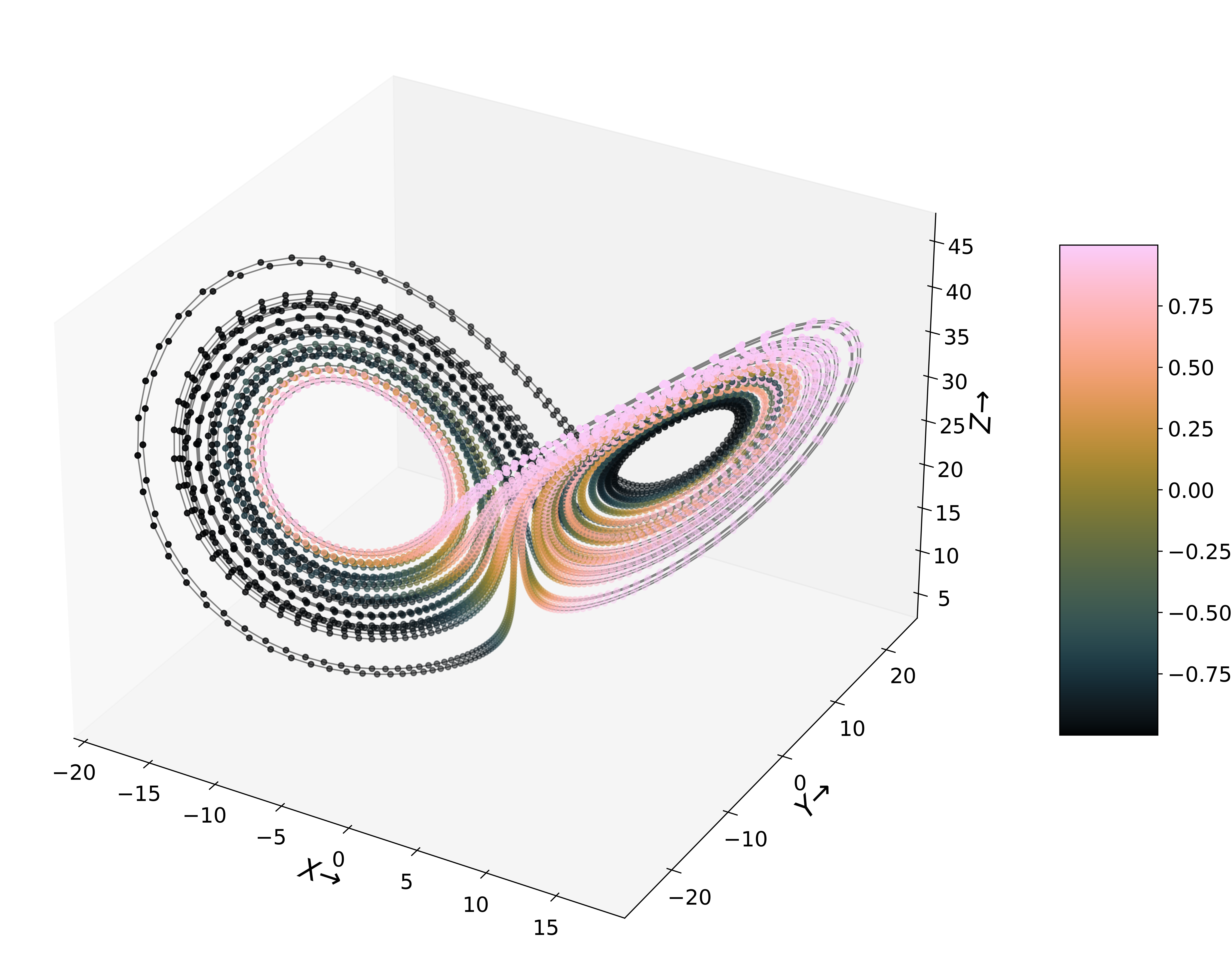
Below we have CLVs of Lorenz-63, which is a 3-dimensional chaotic ODE system and has a butterfly shaped attractor for a specific set of values of the parameters $(\sigma,\rho,\beta)=(10,28,8/3)$. We plot the 1st CLV and 2nd CLV for their first two components. The ODE for this system is written below. $$ \frac{dx}{dt}=\sigma \left(y-x\right), \frac{dy}{dt}=x\left(\rho-z\right)-y, \frac{dz}{dt}=xy-\beta z $$
Here is a picture of the attractor of the Lorenz-63 system, where the angle between the first and the second clv is shown. Whenever the trajectory moves from the right to the left wing of this butterfly attractor, the first two CLVs become parallel and for left to right they become anti-parallel.
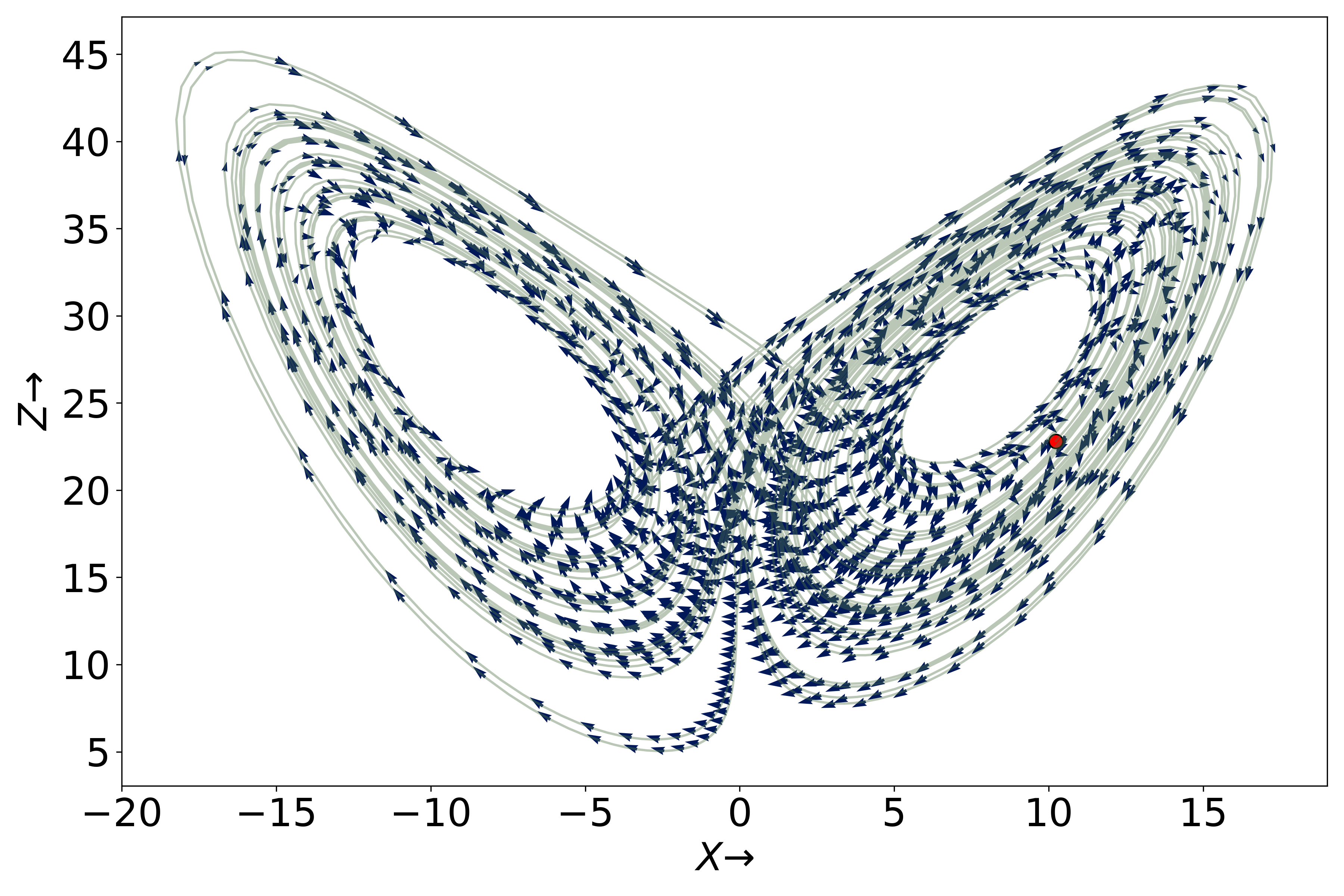
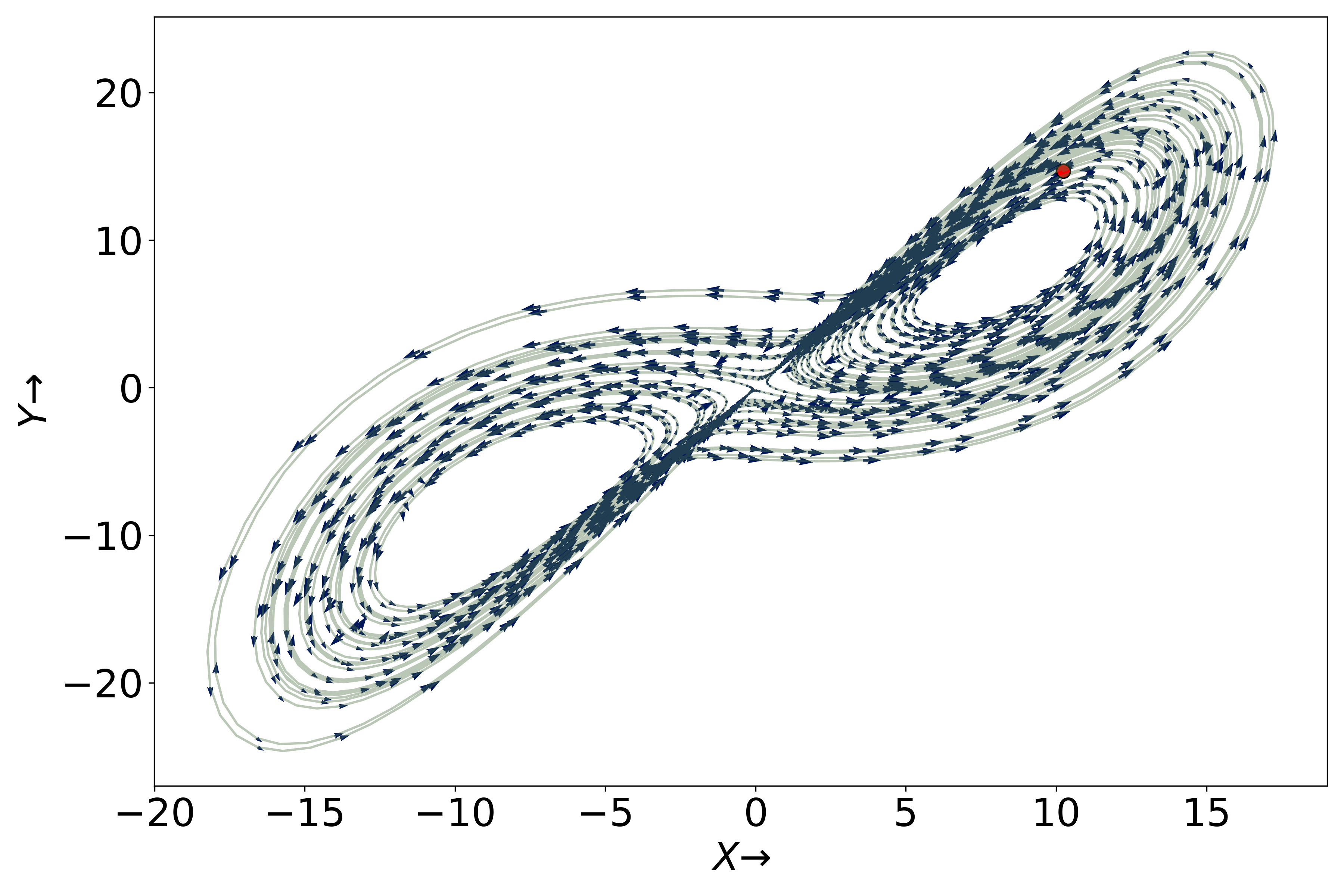
Plotting the first two components of the vectors is shown below. An interesting thing to note is that there is a gradual change in the directions of the vectors as we move along the trajectory. Moreover, two nearby points on the attractor have some degree of similarity in terms of the directions of the vectors themselves. Since there computation needs an underlying trajectory, some degree of their smoothness may be of some merit when applying some supervised machine learning methods to learn and predict them.
Below is CLV 1, where we only ploy the X and Z component of the vectors.

Below is CLV 2, where we only ploy the X and Z component of the vectors.

Research Problem
The specific questions which we ask about lyapunov vectors and exponents in context of the filtering problem are as follows:
- How sensitive are the backward and covariant lyapunov vectors and the corresponding exponents to perturbations in the underlying trajectory?
- Under what conditions can one recover them from a filter estimated trajectory instead of the true trajectory of the dynamical system?
- How robust are unstable subspaces to the perturbation strength $\sigma$, and are they more robust than the individual vectors themselves?
The above questions are relevant to both nonlinear dynamics and weather forecasting techniques since the underlying true trajectory is not accessible but are required in order to compute the LVs. What one can do best is to use the best estimate of the true state given observations upto a certain time. This comes with a caveat that the filter estimates or the analysis mean over time is not a dynamical trajectory of the system, i.e. there is not intial condition on the model which can generate this trajectory starting from a certain initial condition. The true trajectory lies near the analysis mean which is quantifies by the error in the estimates themselves. The sensitivity of BLVs and CLVs for a particular system tells us the limitations of what can be reconstructed from the filter estimates themselves.
In high-dimensions, I used Lorenz-96 in order to explore dimensional dependence added to the sensitivity problem. Another interesting directions is using principle angles(to cite), which summarize the angle between two different subspaces, and seeing how they change with $\sigma$, which I found to be more robust than the individual vectors themselves. Such study is useful in context of problems where subspaces are more important than the individual vectors themselves. Once the above results are interpretable, we can then reconstruct lyapunov vectors from a filter generated trajectory using partial and noisy observations and a model.
Possible directions for future work
A set of directions for future work directly following the current work are:
- Combining the ideas of assimilation in unstable subspace and stability, are the two related to each other?
- Capturing the effect of model errors themselves on the computed lyapunov vectors.
- Using the subspaces computed from reanalysis data which can be used to restrict the uncertainty in forecasts and analysis in data assimilation cycles.
- The degree of similarity in the lyapunov vectors between two nearby points on the attractor in phase space which may be important machine learning methods trained on vectors computed once along a trajectory be used to predict vectors at neaby points in the phase space.
- Studying structure of CLVs for discretized PDE systems such as Kuramoto-sivashinksy equation which has a finite dimensional attractor to shed light on CLV localization problem.
references
[1] Roy, Shashank and Apte, Amit, A note on sensitivity of Lyapunov vectors to trajectory perturbations
[2] Pazo, Diego and Szendro, Ivan G. and Lopez, Juan M. and Rodriguez, Miguel, A.Structure of characteristic Lyapunov vectors in spatiotemporal chaos, 2008.
[3] Vannitsem and Lucarini,Statistical and dynamical properties of covariant lyapunov vectors in a coupled atmosphere-ocean model-multiscale effects, geometric degeneracy, and error dynamics,Journal of Physics A: Mathematical and Theoretical, 2016.